Table of Contents

What is SQL? The Language of Databases

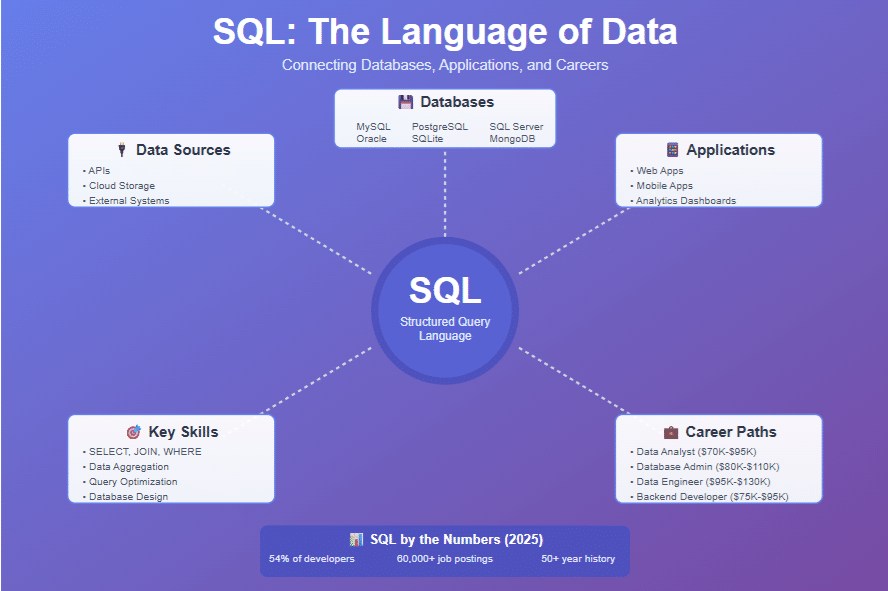
SQL (Structured Query Language) is the standard programming language for managing and manipulating relational databases. Think of SQL syntax basics as the universal language that lets you “talk” to databases—whether you’re asking questions about your data, adding new information, updating existing records, or removing outdated entries.

What Makes SQL Special?

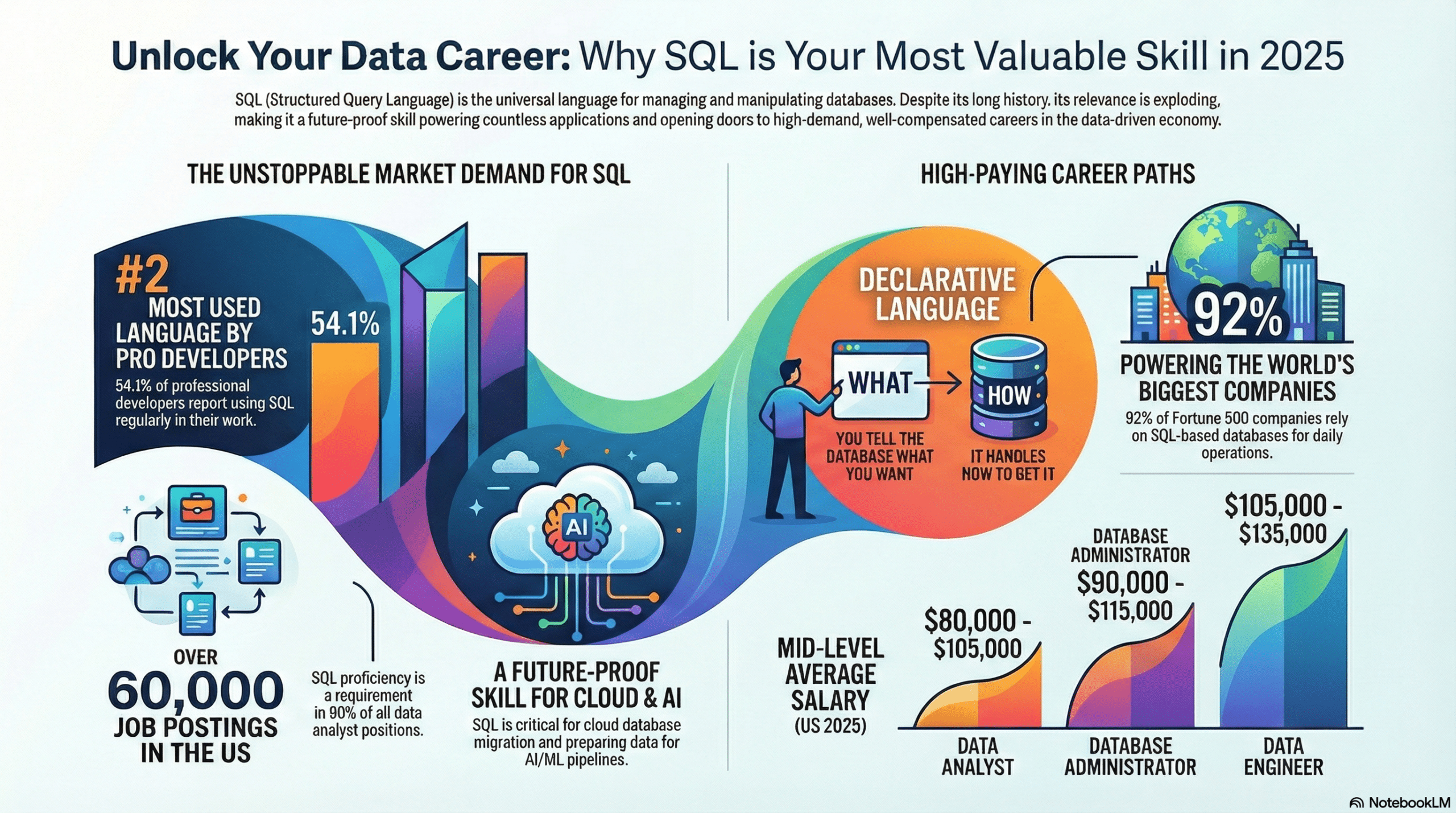
Unlike programming languages like Python or JavaScript that tell computers what to do step-by-step, SQL is a declarative language—you tell it what you want, and the database figures out how to get it for you.

Real-World Analogy:

Traditional Programming (Imperative):
“Go to the library, walk to aisle 3, find shelf 5,
look for books from 2020-2024, bring me the ones about Python”

SQL (Declarative):
“Give me all Python books published between 2020 and 2024”

Where is SQL Used?

SQL powers virtually every data-driven application you use daily:

Social Media: Facebook, Instagram, Twitter use SQL to store and retrieve your posts, messages, and connections

E-commerce: Amazon, eBay query product catalogs, process orders, track inventory

Banking: Banks use SQL for transactions, account management, fraud detection

Healthcare: Hospitals manage patient records, appointments, medical history

Streaming Services: Netflix, Spotify recommend content based on SQL queries analyzing your viewing/listening history

Business Intelligence: Companies analyze sales, customer behavior, financial data

Market Reality 2025: According to the 2024 Stack Overflow Developer Survey, SQL is the second most popular language among professional developers, with 54.1% using it regularly. Despite being created in the 1970s, SQL remains more relevant than ever.

Why Learn SQL in 2025? Market Demand & Career Opportunities

The Unstoppable Demand for SQL Skills

Job Market Statistics 2024-2025:

Over 60,000 SQL-related job postings in the US alone (LinkedIn, 2024)

80% of data analyst positions require SQL proficiency

Average salary increase: 15-25% when you add SQL to your skillset

92% of Fortune 500 companies use SQL-based databases

Salary Ranges by Role (US Market 2025)

Role	Entry-Level	Mid-Level	Senior-Level
Data Analyst	$65,000 – $80,000	$80,000 – $105,000	$105,000 – $130,000
Database Administrator	$70,000 – $90,000	$90,000 – $115,000	$115,000 – $145,000
Data Engineer	$85,000 – $105,000	$105,000 – $135,000	$135,000 – $170,000
Business Intelligence Analyst	$70,000 – $85,000	$85,000 – $110,000	$110,000 – $140,000
Backend Developer (SQL)	$75,000 – $95,000	$95,000 – $125,000	$125,000 – $155,000

Why SQL is Future-Proof

1. Cloud Database Explosion: Over 80% of large enterprises are migrating to cloud platforms (AWS, Azure, Google Cloud), all of which use SQL-based databases.

2. AI Integration: The 2024 Forrester report notes that SQL is key to making AI and machine learning work with databases. Modern ML pipelines rely heavily on SQL for data preparation.

3. Universal Skill: Whether you work in tech, finance, healthcare, retail, or government—SQL is required. It’s the closest thing to a “universal language” in the data world

4. Low Learning Curve, High ROI: You can learn enough SQL to be productive in 2-4 weeks of focused study, yet the career benefits last a lifetime.

SQL Syntax Fundamentals: The Building Blocks

Understanding SQL Statement Structure

Every SQL query follows a specific structure. Let’s break down the anatomy:

SELECT column1, column2, column3
FROM table_name
WHERE condition
ORDER BY column1 DESC;

Components:

SELECT: Specifies which columns you want to retrieve
FROM: Specifies which table(s) to query
WHERE: Filters rows based on conditions (optional)
ORDER BY: Sorts results (optional)
Semicolon (;): Marks the end of the statement

SQL Syntax Rules

Rule 1: SQL is NOT Case-Sensitive (for keywords)

-- These are all equivalent:
SELECT * FROM customers;
select * from customers;
Select * From Customers;

Best Practice: Use UPPERCASE for SQL keywords, lowercase for table/column names

-- Good:
SELECT customer_name, email FROM customers;

-- Also acceptable:
select customer_name, email from customers;

Rule 2: White Space Doesn’t Matter (to SQL)

-- One line:
SELECT name FROM users WHERE age > 25;

-- Multiple lines (more readable):
SELECT name
FROM users
WHERE age > 25;

Rule 3: Semicolons End Statements

-- Single query:
SELECT * FROM products;

-- Multiple queries:
SELECT * FROM customers;
SELECT * FROM orders;
SELECT * FROM products;

Rule 4: Comments Explain Code

-- This is a single-line comment

/* This is a multi-line comment */

SELECT name  -- Get customer names
FROM customers
WHERE status = 'active';  -- Only active customers

SQL Data Types (Quick Reference)

Category	Data Types	Example
Text	VARCHAR, CHAR, TEXT	‘John Smith’, ‘user@email.com‘
Numbers	INT, BIGINT, DECIMAL, FLOAT	42, 1000000, 99.99, 3.14159
Date/Time	DATE, TIME, DATETIME, TIMESTAMP	‘2024-11-28′, ’14:30:00’, ‘2024-11-28 14:30:00’
Boolean	BOOLEAN, BIT	TRUE, FALSE, 0, 1
Binary	BLOB, BINARY	Image files, PDFs

SELECT Statement: Retrieving Data

The SELECT statement is the most frequently used SQL command. It’s how you ask the database to show you data.

Basic SELECT Syntax

SELECT column_name(s)
FROM table_name;

Example Database Schema

Let’s work with a simple employees table:

employees table:
+-------------+------------+-----------+----------------------+------------+--------+------------+
| employee_id | first_name | last_name | email                | department | salary | hire_date  |
+-------------+------------+-----------+----------------------+------------+--------+------------+
| 1           | John       | Smith     | john.smith@co.com    | Sales      | 65000  | 2022-03-15 |
| 2           | Sarah      | Johnson   | sarah.j@co.com       | Marketing  | 72000  | 2021-07-22 |
| 3           | Michael    | Brown     | m.brown@co.com       | IT         | 85000  | 2020-01-10 |
| 4           | Emily      | Davis     | emily.d@co.com       | Sales      | 68000  | 2023-05-18 |
| 5           | David      | Wilson    | d.wilson@co.com      | IT         | 92000  | 2019-11-30 |
+-------------+------------+-----------+----------------------+------------+--------+------------+

SELECT All Columns

The asterisk (*) selects all columns:

SELECT *
FROM employees;

Result: Returns all columns and all rows from the employees table.

When to use: Quick exploration, checking table structure When NOT to use: Production code (slow, wastes bandwidth)

SELECT Specific Columns

SELECT first_name, last_name, department
FROM employees;

Result:

+------------+-----------+------------+
| first_name | last_name | department |
+------------+-----------+------------+
| John       | Smith     | Sales      |
| Sarah      | Johnson   | Marketing  |
| Michael    | Brown     | IT         |
| Emily      | Davis     | Sales      |
| David      | Wilson    | IT         |
+------------+-----------+------------+

Best Practice: Always select only the columns you need.

Column Aliases (Renaming Columns)

SELECT 
    first_name AS "First Name",
    last_name AS "Last Name",
    salary AS "Annual Salary"
FROM employees;

Result:

+------------+-----------+---------------+
| First Name | Last Name | Annual Salary |
+------------+-----------+---------------+
| John       | Smith     | 65000         |
| Sarah      | Johnson   | 72000         |
| Michael    | Brown     | 85000         |
+------------+-----------+---------------+

Use AS keyword to make column names more readable in results.

Calculated Columns

SELECT 
    first_name,
    last_name,
    salary,
    salary * 1.10 AS "Salary After 10% Raise",
    salary / 12 AS "Monthly Salary"
FROM employees;

Result:

+------------+-----------+--------+-------------------------+----------------+
| first_name | last_name | salary | Salary After 10% Raise  | Monthly Salary |
+------------+-----------+--------+-------------------------+----------------+
| John       | Smith     | 65000  | 71500.00               | 5416.67        |
| Sarah      | Johnson   | 72000  | 79200.00               | 6000.00        |
| Michael    | Brown     | 85000  | 93500.00               | 7083.33        |
+------------+-----------+--------+-------------------------+----------------+

String Concatenation

Combine text columns:

SELECT 
    CONCAT(first_name, ' ', last_name) AS "Full Name",
    email,
    department
FROM employees;

Result:

+----------------+----------------------+------------+
| Full Name      | email                | department |
+----------------+----------------------+------------+
| John Smith     | john.smith@co.com    | Sales      |
| Sarah Johnson  | sarah.j@co.com       | Marketing  |
| Michael Brown  | m.brown@co.com       | IT         |
+----------------+----------------------+------------+

DISTINCT: Removing Duplicates

SELECT DISTINCT department
FROM employees;

Result:

+------------+
| department |
+------------+
| Sales      |
| Marketing  |
| IT         |
+------------+

Without DISTINCT, you’d see “Sales” and “IT” listed multiple times.

WHERE Clause: Filtering Your Results

The WHERE clause filters rows based on specified conditions. It’s like asking: “Show me only the data that matches these criteria.”

Basic WHERE Syntax

SELECT column_name(s)
FROM table_name
WHERE condition;

Comparison Operators

Operator	Meaning	Example
`=`	Equal to	`WHERE salary = 65000`
`!=` or `<>`	Not equal to	`WHERE department != 'Sales'`
`>`	Greater than	`WHERE salary > 70000`
`<`	Less than	`WHERE salary < 80000`
`>=`	Greater than or equal	`WHERE salary >= 70000`
`<=`	Less than or equal	`WHERE salary <= 80000`

Filtering Examples

Example 1: Exact Match

SELECT first_name, last_name, department, salary
FROM employees
WHERE department = 'IT';

Result:

+------------+-----------+------------+--------+
| first_name | last_name | department | salary |
+------------+-----------+------------+--------+
| Michael    | Brown     | IT         | 85000  |
| David      | Wilson    | IT         | 92000  |
+------------+-----------+------------+--------+

Example 2: Numeric Comparison

SELECT first_name, last_name, salary
FROM employees
WHERE salary > 70000;

Result:

+------------+-----------+--------+
| first_name | last_name | salary |
+------------+-----------+--------+
| Sarah      | Johnson   | 72000  |
| Michael    | Brown     | 85000  |
| David      | Wilson    | 92000  |
+------------+-----------+--------+

Logical Operators: AND, OR, NOT

AND: Both conditions must be true

SELECT first_name, last_name, department, salary
FROM employees
WHERE department = 'IT' 
AND salary > 85000;

Result: Only David Wilson (IT department AND salary > 85000)

OR: At least one condition must be true

SELECT first_name, last_name, department
FROM employees
WHERE department = 'Sales' 
OR department = 'Marketing';

Result: Returns employees in Sales OR Marketing (both departments)

NOT: Negates a condition

SELECT first_name, last_name, department
FROM employees
WHERE NOT department = 'IT';

Result: Returns all employees EXCEPT those in IT

Combining Multiple Conditions

SELECT first_name, last_name, department, salary
FROM employees
WHERE (department = 'Sales' OR department = 'IT')
  AND salary >= 70000;

Explanation:

Must work in Sales OR IT (parentheses ensure OR is evaluated first)
AND must earn at least $70,000

Result: Sarah Johnson (Marketing, 72K) is excluded because she’s not in Sales/IT. John Smith (Sales, 65K) is excluded because salary < 70K.

BETWEEN: Range Filtering

SELECT first_name, last_name, salary
FROM employees
WHERE salary BETWEEN 65000 AND 80000;

Equivalent to:

WHERE salary >= 65000 AND salary <= 80000

Result:

+------------+-----------+--------+
| first_name | last_name | salary |
+------------+-----------+--------+
| John       | Smith     | 65000  |
| Sarah      | Johnson   | 72000  |
| Emily      | Davis     | 68000  |
+------------+-----------+--------+

IN: Multiple Values

SELECT first_name, last_name, department
FROM employees
WHERE department IN ('Sales', 'Marketing', 'HR');

Equivalent to:

WHERE department = 'Sales' 
   OR department = 'Marketing' 
   OR department = 'HR'

Much cleaner syntax!

LIKE: Pattern Matching

Wildcards:

% = any sequence of characters (including zero characters)
_ = exactly one character

Example 1: Starts with

SELECT first_name, last_name
FROM employees
WHERE first_name LIKE 'J%';

Matches: John (starts with J) Doesn’t match: Sarah, Michael, Emily, David

Example 2: Ends with

SELECT first_name, last_name
FROM employees
WHERE last_name LIKE '%son';

Matches: Johnson, Wilson (end with “son”)

Example 3: Contains

SELECT first_name, email
FROM employees
WHERE email LIKE '%@co.com%';

Matches: All emails containing “@co.com”

Example 4: Exact position

SELECT first_name
FROM employees
WHERE first_name LIKE '_____';  -- Exactly 5 letters

Matches: Emily, David, Sarah (5-letter names) Doesn’t match: John (4 letters), Michael (7 letters)

IS NULL / IS NOT NULL

-- Find employees with no email
SELECT first_name, last_name
FROM employees
WHERE email IS NULL;

-- Find employees with email
SELECT first_name, last_name, email
FROM employees
WHERE email IS NOT NULL;

Important: Never use = NULL or != NULL. Always use IS NULL or IS NOT NULL.

ORDER BY: Sorting Data

ORDER BY sorts query results in ascending (ASC) or descending (DESC) order.

Basic ORDER BY Syntax

SELECT column_name(s)
FROM table_name
ORDER BY column_name [ASC|DESC];

Sorting Examples

Example 1: Ascending Order (Default)

SELECT first_name, last_name, salary
FROM employees
ORDER BY salary;  -- ASC is default

Result (lowest to highest salary):

+------------+-----------+--------+
| first_name | last_name | salary |
+------------+-----------+--------+
| John       | Smith     | 65000  |
| Emily      | Davis     | 68000  |
| Sarah      | Johnson   | 72000  |
| Michael    | Brown     | 85000  |
| David      | Wilson    | 92000  |
+------------+-----------+--------+

Example 2: Descending Order

SELECT first_name, last_name, salary
FROM employees
ORDER BY salary DESC;

Result (highest to lowest salary):

+------------+-----------+--------+
| first_name | last_name | salary |
+------------+-----------+--------+
| David      | Wilson    | 92000  |
| Michael    | Brown     | 85000  |
| Sarah      | Johnson   | 72000  |
| Emily      | Davis     | 68000  |
| John       | Smith     | 65000  |
+------------+-----------+--------+

Multiple Column Sorting

SELECT first_name, last_name, department, salary
FROM employees
ORDER BY department ASC, salary DESC;

How it works:

First, sort by department (alphabetically)
Within each department, sort by salary (highest to lowest)

Result:

+------------+-----------+------------+--------+
| first_name | last_name | department | salary |
+------------+-----------+------------+--------+
| David      | Wilson    | IT         | 92000  |  ← IT dept, higher salary
| Michael    | Brown     | IT         | 85000  |  ← IT dept, lower salary
| Sarah      | Johnson   | Marketing  | 72000  |
| Emily      | Davis     | Sales      | 68000  |  ← Sales, higher salary
| John       | Smith     | Sales      | 65000  |  ← Sales, lower salary
+------------+-----------+------------+--------+

Sorting by Column Position

SELECT first_name, last_name, salary
FROM employees
ORDER BY 3 DESC;  -- 3 = third column (salary)

Not recommended (hard to read), but useful to know.

JOIN Operations: Combining Tables

JOINs are how you combine data from multiple tables based on related columns. This is where SQL becomes truly powerful.

Sample Tables for JOIN Examples

employees table:

+-------------+------------+-----------+---------------+
| employee_id | first_name | last_name | department_id |
+-------------+------------+-----------+---------------+
| 1           | John       | Smith     | 10            |
| 2           | Sarah      | Johnson   | 20            |
| 3           | Michael    | Brown     | 30            |
| 4           | Emily      | Davis     | 10            |
| 5           | David      | Wilson    | NULL          |
+-------------+------------+-----------+---------------+

departments table:

+---------------+-----------------+
| department_id | department_name |
+---------------+-----------------+
| 10            | Sales           |
| 20            | Marketing       |
| 30            | IT              |
| 40            | HR              |
+---------------+-----------------+

INNER JOIN: Matching Rows Only

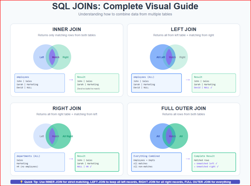
Returns only rows where there’s a match in BOTH tables.

SELECT 
    e.first_name,
    e.last_name,
    d.department_name
FROM employees e
INNER JOIN departments d 
    ON e.department_id = d.department_id;

Result:

+------------+-----------+-----------------+
| first_name | last_name | department_name |
+------------+-----------+-----------------+
| John       | Smith     | Sales           |
| Sarah      | Johnson   | Marketing       |
| Michael    | Brown     | IT              |
| Emily      | Davis     | Sales           |
+------------+-----------+-----------------+

Notice:

David Wilson is EXCLUDED (no matching department_id)
HR department is EXCLUDED (no employees in it)

LEFT JOIN (LEFT OUTER JOIN): All from Left Table

Returns ALL rows from the left table, plus matching rows from the right table. If no match, NULL values appear.

SELECT 
    e.first_name,
    e.last_name,
    d.department_name
FROM employees e
LEFT JOIN departments d 
    ON e.department_id = d.department_id;

Result:

+------------+-----------+-----------------+
| first_name | last_name | department_name |
+------------+-----------+-----------------+
| John       | Smith     | Sales           |
| Sarah      | Johnson   | Marketing       |
| Michael    | Brown     | IT              |
| Emily      | Davis     | Sales           |
| David      | Wilson    | NULL            |  ← No department match
+------------+-----------+-----------------+

Use case: “Show me all employees, including those not assigned to a department”

RIGHT JOIN (RIGHT OUTER JOIN): All from Right Table

Returns ALL rows from the right table, plus matching rows from the left table.

SELECT 
    e.first_name,
    e.last_name,
    d.department_name
FROM employees e
RIGHT JOIN departments d 
    ON e.department_id = d.department_id;

Result:

+------------+-----------+-----------------+
| first_name | last_name | department_name |
+------------+-----------+-----------------+
| John       | Smith     | Sales           |
| Emily      | Davis     | Sales           |
| Sarah      | Johnson   | Marketing       |
| Michael    | Brown     | IT              |
| NULL       | NULL      | HR              |  ← No employees in HR
+------------+-----------+-----------------+

Use case: “Show me all departments, including those with no employees”

FULL OUTER JOIN: All from Both Tables

Returns ALL rows from both tables. Where there’s no match, NULL values appear.

SELECT 
    e.first_name,
    e.last_name,
    d.department_name
FROM employees e
FULL OUTER JOIN departments d 
    ON e.department_id = d.department_id;

Result:

+------------+-----------+-----------------+
| first_name | last_name | department_name |
+------------+-----------+-----------------+
| John       | Smith     | Sales           |
| Sarah      | Johnson   | Marketing       |
| Michael    | Brown     | IT              |
| Emily      | Davis     | Sales           |
| David      | Wilson    | NULL            |  ← Employee with no dept
| NULL       | NULL      | HR              |  ← Dept with no employees
+------------+-----------+-----------------+

Use case: “Show me everything—all employees and all departments”

Multiple JOIN Example

SELECT 
    e.first_name,
    e.last_name,
    d.department_name,
    p.project_name
FROM employees e
INNER JOIN departments d 
    ON e.department_id = d.department_id
INNER JOIN projects p 
    ON e.employee_id = p.employee_id;

You can chain multiple JOINs to combine 3, 4, or more tables!

Aggregate Functions: Summarizing Data

Aggregate functions perform calculations on multiple rows and return a single result.

Common Aggregate Functions

Function	Purpose	Example
`COUNT()`	Count rows	`COUNT(*)` or `COUNT(column_name)`
`SUM()`	Add values	`SUM(salary)`
`AVG()`	Calculate average	`AVG(salary)`
`MIN()`	Find minimum	`MIN(salary)`
`MAX()`	Find maximum	`MAX(salary)`

COUNT: Counting Rows

-- Count all employees
SELECT COUNT(*) AS total_employees
FROM employees;

Result:

+------------------+
| total_employees  |
+------------------+
| 5                |
+------------------+

-- Count employees with email (NULL values excluded)
SELECT COUNT(email) AS employees_with_email
FROM employees;

-- Count distinct departments
SELECT COUNT(DISTINCT department) AS number_of_departments
FROM employees;

SUM: Adding Values

SELECT SUM(salary) AS total_payroll
FROM employees;

Result:

+---------------+
| total_payroll |
+---------------+
| 382000        |
+---------------+

AVG: Calculating Average

SELECT AVG(salary) AS average_salary
FROM employees;

Result:

+----------------+
| average_salary |
+----------------+
| 76400.00       |
+----------------+

-- Round to 2 decimal places
SELECT ROUND(AVG(salary), 2) AS average_salary
FROM employees;

MIN and MAX: Finding Extremes

SELECT 
    MIN(salary) AS lowest_salary,
    MAX(salary) AS highest_salary,
    MAX(salary) - MIN(salary) AS salary_range
FROM employees;

Result:

+---------------+----------------+--------------+
| lowest_salary | highest_salary | salary_range |
+---------------+----------------+--------------+
| 65000         | 92000          | 27000        |
+---------------+----------------+--------------+

Combining Multiple Aggregates

SELECT 
    COUNT(*) AS total_employees,
    SUM(salary) AS total_payroll,
    AVG(salary) AS average_salary,
    MIN(salary) AS min_salary,
    MAX(salary) AS max_salary
FROM employees;

Result:

+------------------+---------------+----------------+------------+------------+
| total_employees  | total_payroll | average_salary | min_salary | max_salary |
+------------------+---------------+----------------+------------+------------+
| 5                | 382000        | 76400.00       | 65000      | 92000      |
+------------------+---------------+----------------+------------+------------+

GROUP BY and HAVING: Grouping Data

GROUP BY groups rows that have the same values in specified columns, allowing you to perform aggregate functions on each group.

GROUP BY Syntax

sql

SELECT column_name, aggregate_function(column_name)
FROM table_name
GROUP BY column_name;

Basic GROUP BY Example

SELECT 
    department,
    COUNT(*) AS employee_count,
    AVG(salary) AS avg_salary
FROM employees
GROUP BY department;

Result:

+------------+----------------+------------+
| department | employee_count | avg_salary |
+------------+----------------+------------+
| Sales      | 2              | 66500.00   |
| Marketing  | 1              | 72000.00   |
| IT         | 2              | 88500.00   |
+------------+----------------+------------+

Explanation: SQL groups all Sales employees together, all Marketing together, etc., then calculates COUNT and AVG for each group.

Multiple Column GROUP BY

SELECT 
    department,
    YEAR(hire_date) AS hire_year,
    COUNT(*) AS employees_hired
FROM employees
GROUP BY department, YEAR(hire_date)
ORDER BY department, hire_year;

Result:

+------------+-----------+------------------+
| department | hire_year | employees_hired  |
+------------+-----------+------------------+
| IT         | 2019      | 1                |
| IT         | 2020      | 1                |
| Marketing  | 2021      | 1                |
| Sales      | 2022      | 1                |
| Sales      | 2023      | 1                |
+------------+-----------+------------------+

HAVING: Filtering Grouped Results

WHERE filters BEFORE grouping HAVING filters AFTER grouping

-- Find departments with average salary > $70,000
SELECT 
    department,
    COUNT(*) AS employee_count,
    AVG(salary) AS avg_salary
FROM employees
GROUP BY department
HAVING AVG(salary) > 70000;

Result:

+------------+----------------+------------+
| department | employee_count | avg_salary |
+------------+----------------+------------+
| Marketing  | 1              | 72000.00   |
| IT         | 2              | 88500.00   |
+------------+----------------+------------+

Sales department excluded because average salary ($66,500) is below $70,000.

WHERE vs HAVING Example

-- WHERE: Filter BEFORE grouping
SELECT 
    department,
    AVG(salary) AS avg_salary
FROM employees
WHERE salary > 70000  -- Only include employees earning > 70K
GROUP BY department;

-- HAVING: Filter AFTER grouping
SELECT 
    department,
    AVG(salary) AS avg_salary
FROM employees
GROUP BY department
HAVING AVG(salary) > 70000;  -- Only show departments with avg > 70K

Key Difference:

WHERE filters individual rows
HAVING filters grouped results

Combining WHERE, GROUP BY, and HAVING

SELECT 
    department,
    COUNT(*) AS employee_count,
    AVG(salary) AS avg_salary
FROM employees
WHERE salary > 60000  -- First: filter rows (exclude low earners)
GROUP BY department   -- Then: group by department
HAVING COUNT(*) > 1   -- Finally: only show departments with 2+ employees
ORDER BY avg_salary DESC;

Execution order:

Filter: Only employees earning > $60,000
Group: By department
Filter groups: Only departments with more than 1 employee
Sort: By average salary (highest first)

INSERT, UPDATE, DELETE: Modifying Data

So far we’ve focused on retrieving data (SELECT). Now let’s learn to modify data.

INSERT: Adding New Rows

Syntax:

INSERT INTO table_name (column1, column2, column3)
VALUES (value1, value2, value3);

Example 1: Insert Single Row

INSERT INTO employees (employee_id, first_name, last_name, email, department, salary, hire_date)
VALUES (6, 'Anna', 'Garcia', 'anna.g@co.com', 'HR', 70000, '2024-11-28');

Example 2: Insert Multiple Rows

INSERT INTO employees (employee_id, first_name, last_name, department, salary, hire_date)
VALUES 
    (7, 'James', 'Miller', 'Sales', 67000, '2024-12-01'),
    (8, 'Lisa', 'Anderson', 'Marketing', 75000, '2024-12-01'),
    (9, 'Robert', 'Taylor', 'IT', 88000, '2024-12-01');

Example 3: Insert with NULL Values

INSERT INTO employees (employee_id, first_name, last_name, department)
VALUES (10, 'Chris', 'Moore', 'Sales');
-- Email, salary, and hire_date will be NULL

UPDATE: Modifying Existing Rows

⚠️ WARNING: Always use WHERE clause with UPDATE or you’ll modify ALL rows!

Syntax:

UPDATE table_name
SET column1 = value1, column2 = value2
WHERE condition;

Example 1: Update Single Row

UPDATE employees
SET salary = 95000
WHERE employee_id = 5;

Example 2: Update Multiple Columns

UPDATE employees
SET 
    salary = 70000,
    department = 'Marketing'
WHERE employee_id = 4;

Example 3: Update Based on Calculation

-- Give 10% raise to IT department
UPDATE employees
SET salary = salary * 1.10
WHERE department = 'IT';

Example 4: Update Multiple Rows

-- Give $5,000 raise to all Sales employees
UPDATE employees
SET salary = salary + 5000
WHERE department = 'Sales';

DELETE: Removing Rows

⚠️ EXTREME WARNING: DELETE without WHERE deletes ALL rows!

Syntax:

DELETE FROM table_name
WHERE condition;

Example 1: Delete Single Row

DELETE FROM employees
WHERE employee_id = 10;

Example 2: Delete Multiple Rows

DELETE FROM employees
WHERE department = 'HR' AND salary < 50000;

Example 3: Delete All Rows (Dangerous!)

-- This deletes EVERYTHING!
DELETE FROM employees;

-- Better: Use TRUNCATE for deleting all rows (faster)
TRUNCATE TABLE employees;

Best Practice: Test with SELECT First

-- Step 1: Test your WHERE clause with SELECT
SELECT * FROM employees WHERE department = 'Temp';

-- Step 2: If results look correct, change SELECT to DELETE
DELETE FROM employees WHERE department = 'Temp';

Common SQL Syntax Mistakes to Avoid

Mistake 1: Forgetting WHERE Clause

-- ❌ WRONG: Updates ALL employees!
UPDATE employees
SET department = 'Sales';

-- ✅ CORRECT: Updates only one employee
UPDATE employees
SET department = 'Sales'
WHERE employee_id = 5;

Mistake 2: Using = with NULL

-- ❌ WRONG: Will return 0 rows
SELECT * FROM employees WHERE email = NULL;

-- ✅ CORRECT: Use IS NULL
SELECT * FROM employees WHERE email IS NULL;

Mistake 3: Forgetting to GROUP BY Selected Columns

-- ❌ WRONG: Error! department not in GROUP BY
SELECT department, COUNT(*), AVG(salary)
FROM employees
GROUP BY employee_id;

-- ✅ CORRECT: All non-aggregated columns must be in GROUP BY
SELECT department, COUNT(*), AVG(salary)
FROM employees
GROUP BY department;

Mistake 4: String Values Without Quotes

-- ❌ WRONG: Sales is not a column, it's a value!
SELECT * FROM employees WHERE department = Sales;

-- ✅ CORRECT: Use quotes for string values
SELECT * FROM employees WHERE department = 'Sales';

Mistake 5: Wrong ORDER of Clauses

-- ❌ WRONG: Clauses in wrong order
SELECT * FROM employees
ORDER BY salary
WHERE department = 'IT';

-- ✅ CORRECT: WHERE before ORDER BY
SELECT * FROM employees
WHERE department = 'IT'
ORDER BY salary;

SQL Clause Order:

SELECT
FROM
WHERE
GROUP BY
HAVING
ORDER BY

Mistake 6: Confusing AND with OR

-- ❌ WRONG: Looking for impossible condition
SELECT * FROM employees
WHERE department = 'Sales' AND department = 'IT';
-- Can't be both Sales AND IT simultaneously!

-- ✅ CORRECT: Use OR for alternatives
SELECT * FROM employees
WHERE department = 'Sales' OR department = 'IT';

Mistake 7: Not Using Aliases for Tables

-- ❌ CONFUSING: Which table has which column?
SELECT first_name, department_name
FROM employees
JOIN departments ON employees.department_id = departments.department_id;

-- ✅ CLEARER: Use table aliases
SELECT e.first_name, d.department_name
FROM employees e
JOIN departments d ON e.department_id = d.department_id;

SQL Query Writing Best Practices

1. Use Meaningful Column and Table Aliases

-- ❌ Poor: Unclear aliases
SELECT a.b, c.d
FROM tbl1 a
JOIN tbl2 c ON a.id = c.fk;

-- ✅ Good: Descriptive aliases
SELECT 
    emp.first_name,
    dept.department_name
FROM employees emp
JOIN departments dept ON emp.department_id = dept.department_id;

2. Always Specify Columns (Avoid SELECT *)

-- ❌ Poor: Selects everything (slow, wastes bandwidth)
SELECT * FROM employees;

-- ✅ Good: Specify needed columns
SELECT employee_id, first_name, last_name, email
FROM employees;

Why it matters:

Faster queries (less data transferred)
Clearer intent (others know what you need)
Future-proof (table structure changes won’t break query)

3. Format for Readability

-- ❌ Poor: Hard to read
SELECT e.first_name,e.last_name,d.department_name,e.salary FROM employees e JOIN departments d ON e.department_id=d.department_id WHERE e.salary>70000 ORDER BY e.salary DESC;

-- ✅ Good: Formatted and readable
SELECT 
    e.first_name,
    e.last_name,
    d.department_name,
    e.salary
FROM employees e
JOIN departments d 
    ON e.department_id = d.department_id
WHERE e.salary > 70000
ORDER BY e.salary DESC;

4. Use Comments to Explain Complex Logic

-- Get top 10 highest-paid employees in each department
-- Excludes employees hired in the last 6 months (probation period)
SELECT 
    e.department,
    e.first_name,
    e.last_name,
    e.salary
FROM employees e
WHERE e.hire_date < DATE_SUB(CURRENT_DATE, INTERVAL 6 MONTH)  -- Exclude recent hires
ORDER BY e.department, e.salary DESC;

5. Test with LIMIT Before Running on Full Dataset

-- First: Test logic on small sample
SELECT * 
FROM large_table
WHERE condition
LIMIT 10;

-- After confirming correctness: Run on full dataset
SELECT * 
FROM large_table
WHERE condition;

6. Use Consistent Naming Conventions

Choose a style and stick with it:

-- Snake case (recommended)
employee_id, first_name, department_name

-- Camel case
employeeId, firstName, departmentName

-- Pascal case
EmployeeId, FirstName, DepartmentName

7. Use Transactions for Critical Data Changes

-- Begin transaction
START TRANSACTION;

-- Make changes
UPDATE employees SET salary = salary * 1.10 WHERE department = 'IT';
DELETE FROM employees WHERE status = 'terminated';

-- Review changes
SELECT * FROM employees WHERE department = 'IT';

-- If satisfied, commit
COMMIT;

-- If something's wrong, rollback
-- ROLLBACK;

8. Always Backup Before Mass DELETE/UPDATE

-- Step 1: Create backup table
CREATE TABLE employees_backup AS
SELECT * FROM employees;

-- Step 2: Perform risky operation
DELETE FROM employees WHERE condition;

-- Step 3: If something went wrong, restore
-- INSERT INTO employees SELECT * FROM employees_backup;

Practice Exercises with Solutions

Test your SQL knowledge with these exercises!

Exercise 1: Basic SELECT

Question: Write a query to select all columns from the employees table for employees in the IT department.

Solution:

SELECT *
FROM employees
WHERE department = 'IT';

Exercise 2: Filtering with Multiple Conditions

Question: Find all employees who work in Sales or Marketing AND earn more than $70,000.

Solution:

SELECT first_name, last_name, department, salary
FROM employees
WHERE (department = 'Sales' OR department = 'Marketing')
  AND salary > 70000;

Exercise 3: Aggregation

Question: Calculate the total payroll (sum of salaries) for each department.

Solution:

SELECT 
    department,
    SUM(salary) AS total_payroll,
    COUNT(*) AS employee_count
FROM employees
GROUP BY department
ORDER BY total_payroll DESC;

Exercise 4: JOIN

Question: List all employees with their department names. Include employees without a department.

Solution:

SELECT 
    e.first_name,
    e.last_name,
    d.department_name
FROM employees e
LEFT JOIN departments d 
    ON e.department_id = d.department_id;

Exercise 5: Complex Query

Question: Find departments where the average salary is above $75,000 and they have more than 1 employee. Sort by average salary.

Solution:

SELECT 
    department,
    COUNT(*) AS employee_count,
    AVG(salary) AS avg_salary
FROM employees
GROUP BY department
HAVING AVG(salary) > 75000 AND COUNT(*) > 1
ORDER BY avg_salary DESC;

Exercise 6: String Manipulation

Question: Find all employees whose last name contains “son” and format their full name as “Last, First”.

Solution:

SELECT 
    CONCAT(last_name, ', ', first_name) AS full_name,
    email,
    department
FROM employees
WHERE last_name LIKE '%son%';

Exercise 7: Date Filtering

Question: Find employees hired in 2023.

Solution:

SELECT 
    first_name,
    last_name,
    hire_date,
    department
FROM employees
WHERE YEAR(hire_date) = 2023;

-- Alternative using BETWEEN:
WHERE hire_date BETWEEN '2023-01-01' AND '2023-12-31';

Exercise 8: Subquery

Question: Find employees earning more than the average salary.

Solution:

SELECT 
    first_name,
    last_name,
    salary
FROM employees
WHERE salary > (SELECT AVG(salary) FROM employees)
ORDER BY salary DESC;

<> SQL Interactive Exercises

Practice SQL with instant feedback

Progress

0/8

Sample Data:

Expected Output:

Your Answer:

Key Learning Points:

Conclusion: Your SQL Learning Journey

Congratulations! You’ve learned the fundamental building blocks of SQL:

✅ SELECT – Retrieving data ✅ WHERE – Filtering rows ✅ ORDER BY – Sorting results ✅ JOIN – Combining tables ✅ Aggregate Functions – Summarizing data ✅ GROUP BY – Grouping and aggregating ✅ INSERT/UPDATE/DELETE – Modifying data

What You Can Do Now

With these SQL basics, you can:

Extract insights from databases

Answer business questions with data

Build reports and dashboards

Qualify for entry-level data analyst positions

Prepare for data science roles

Your Next Steps

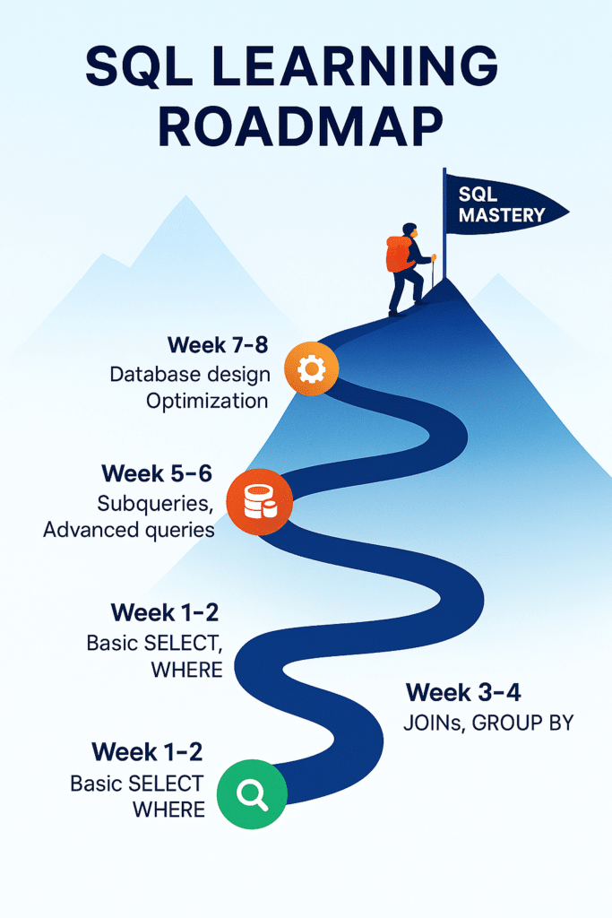
Week 1-2: Practice these basics daily

Complete 10-15 SQL exercises on LeetCode, HackerRank, or SQLZoo
Work with sample databases (TechCorpCompany,Northwind, AdventureWorks)

Week 3-4: Learn intermediate concepts

Subqueries and nested queries
Window functions (ROW_NUMBER, RANK, LAG, LEAD)
CASE statements
CTEs (Common Table Expressions)

Week 5-6: Advanced topics

Indexes and query optimization
Stored procedures and functions
Triggers and views
Transactions and ACID properties

Week 7-8: Real-world projects

Build a personal project (movie database, expense tracker)
Contribute to open-source projects
Create a portfolio on GitHub
Apply for data analyst positions

Recommended Learning Resources

Free Platforms:

SQLZoo – Interactive SQL tutorial

Mode Analytics SQL Tutorial – Business-focused examples

HackerRank SQL – Practice problems

W3Schools SQL Tutorial – Quick reference

Paid Courses (Worth It):

DataCamp – Introduction to SQL ($25/month)

Coursera – SQL for Data Science ($49/month)

Udemy – The Complete SQL Bootcamp (often on sale for $15)

Practice Databases:

Northwind (classic sales database)
AdventureWorks (Microsoft sample database)
Chinook (digital media store)
Sakila (DVD rental store)

Final Thoughts

SQL is one of the most valuable skills you can learn in 2026. Unlike programming languages that come and go, SQL has remained relevant for 50+ years and shows no signs of slowing down.

The best way to learn SQL is by doing. Don’t just read—write queries, make mistakes, debug them, and learn from the process.

Start with 30 minutes of practice daily. In 8 weeks, you’ll be writing complex queries confidently. In 6 months, you’ll be helping colleagues solve data problems. In a year, SQL could transform your career.

Your journey starts with your very next query. Open a SQL editor and try the examples in this guide. The data world is waiting for you!

Post Views: 660